理论基础

简介

自编码器是一种能够通过无监督学习,学到输入数据高效表示的人工神经网络。输入数据的这一高效表示称为编码(codings),其维度一般远小于输入数据,使得自编码器可用于降维。更重要的是,自编码器可作为强大的特征检测器(feature detectors),应用于深度神经网络的预训练。此外,自编码器还可以随机生成与训练数据类似的数据,这被称作生成模型(generative model)。比如,可以用人脸图片训练一个自编码器,它可以生成新的图片。

自编码器通过简单地学习将输入复制到输出来工作。这一任务(就是输入训练数据, 再输出训练数据的任务)听起来似乎微不足道,但通过不同方式对神经网络增加约束,可以使这一任务变得极其困难。比如,可以限制内部表示的尺寸(这就实现降维了),或者对训练数据增加噪声并训练自编码器使其能恢复原有。这些限制条件防止自编码器机械地将输入复制到输出,并强制它学习数据的高效表示。

特点

自动编码器 (AutoEncoder) 最开始作为一种数据的压缩方法,其特点有:

(1)跟数据相关程度很高,这意味着自动编码器只能压缩与训练数据相似的数据,这个其实比较显然,因为使用神经网络提取的特征一般是高度相关于原始的训练集,使用人脸训练出来的自动编码器在压缩自然界动物的图片是表现就会比较差,因为它只学习到了人脸的特征,而没有能够学习到自然界图片的特征;那么在航空航天方面,自然我们要处理一些高清的精密仪器或者系统的图像数据,我们不想直接用神经网络来提取特征,维度会很高,所以可以使用自动编码器先对图像做压缩降维处理。

(2)压缩后数据是有损的,这是因为在降维的过程中不可避免的要丢失掉信息;那么图像数据尽管有损,但也保存了绝大多数信息,从而大幅度提升模型训练效率。

结构

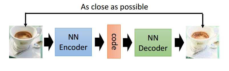
从上面的图中,我们能够看到两个部分,第一个部分是编码器 (Encoder),第二个部分是解码器 (Decoder),编码器和解码器都可以是任意的模型,通常我们使用神经网络模型作为编码器和解码器。输入的数据经过神经网络降维到一个编码 (code),接着又通过另外一个神经网络去解码得到一个与输入原数据一模一样的生成数据,然后通过去比较这两个数据,最小化他们之间的差异来训练这个网络中编码器和解码器的参数。当这个过程训练完之后,我们可以拿出这个解码器,随机传入一个编码 (code),希望通过解码器能够生成一个和原数据差不多的数据,上面这种图这个例子就是希望能够生成一张差不多的图片。

那么我们这里主要介绍通过 TensorFlow 的框架来实现下面三个实例的构建:

  • 基本自编码器的实现
  • 图片去噪自编码器的实现
  • 异常检测

自编码器实际上是一个特殊的神经网络,被训练去“复制”其输入并转化成输出。举个例子,给定一个手写的数字,AE 首先对图片进行编码,使其1变成一个低维的隐变量表达,然后再通过对其解码重构,返还成图片的形式作为输出,那么为什么要这么做呢?我们要做的不是去完全复制图片,而是想办法把原来的输入中的重要特征提取出来,然后重构成一个更低维度的“复制品”,目的是在降低数据维度的情况下,尽量少的损失输入信息,并尽量多的提取特征,也就是极小化重构误差(reconstruction error)。

实例

可能现在你还是不理解编码和解码是什么意思,那么来举个例子。

下面有两组数字,哪组更容易记忆呢?

  • 40, 27, 25, 36, 81, 57, 10, 73, 19, 68
  • 50, 25, 76, 38, 19, 58, 29, 88, 44, 22, 11, 34, 17, 52, 26, 13, 40, 20

乍一看可能觉得第一行数字更容易记忆,毕竟更短。但仔细观察就会发现,第二组数字是有规律的:偶数后面是其二分之一,奇数后面是其三倍加一(这就是著名的hailstone sequence)。如果识别出了这一模式,第二组数据只需要记住这两个规则、第一个数字、以及序列长度。如果你的记忆能力超强,可以记住很长的随机数字序列,那你可能就不会去关心一组数字是否存在规律了。所以我们要对自编码器增加约束来强制它去探索数据中的模式。

记忆(memory)、感知(perception)、和模式匹配(pattern matching)的关系在1970s早期就被William Chase和Herbert Simon研究过。他们发现国际象棋大师观察棋盘5秒,就能记住所有棋子的位置,而常人是无法办到的。但棋子的摆放必须是实战中的棋局(也就是棋子存在规则,就像第二组数字),棋子随机摆放可不行(就像第一组数字)。象棋大师并不是记忆力优于我们,而是经验丰富,很擅于识别象棋模式,从而高效地记忆棋局。

和棋手的记忆模式类似,一个自编码器接收输入,将其转换成高效的内部表示,然后再输出输入数据的类似物。自编码器通常包括两部分:encoder(也称为识别网络)将输入转换成内部表示,decoder(也称为生成网络)将内部表示转换成输出。(如下图)

正如上图所示,自编码器的结构和多层感知机类似,除了输入神经元和输出神经元的个数相等。在上图的例子中,自编码器只有一个包含两个神经元的隐层(encoder),以及包含3个神经元的输出层(decoder)。输出是在设法重建输入,损失函数是重建损失(reconstruction loss)。


TensorFlow 简单实现

1. 调包

In [1]:
import matplotlib.pyplot as plt # 画图
import numpy as np # 数组处理
import pandas as pd # 数据集处理
import tensorflow as tf # tf框架

from sklearn.metrics import accuracy_score, precision_score, recall_score # 评估方法
from sklearn.model_selection import train_test_split # 训练集测试集分割
from tensorflow.keras import layers, losses # 建立神经网络
from tensorflow.keras.datasets import fashion_mnist # mnist数据集获取
from tensorflow.keras.models import Model # 搭建模型

2. 载入数据(数据预处理)

In [2]:
(x_train, _), (x_test, _) = fashion_mnist.load_data()

x_train = x_train.astype('float32') / 255.
x_test = x_test.astype('float32') / 255.

print (x_train.shape)
print (x_test.shape)
Downloading data from https://storage.googleapis.com/tensorflow/tf-keras-datasets/train-labels-idx1-ubyte.gz
32768/29515 [=================================] - 0s 2us/step
Downloading data from https://storage.googleapis.com/tensorflow/tf-keras-datasets/train-images-idx3-ubyte.gz
26427392/26421880 [==============================] - 67s 3us/step
Downloading data from https://storage.googleapis.com/tensorflow/tf-keras-datasets/t10k-labels-idx1-ubyte.gz
8192/5148 [===============================================] - 0s 0s/step
Downloading data from https://storage.googleapis.com/tensorflow/tf-keras-datasets/t10k-images-idx3-ubyte.gz
4423680/4422102 [==============================] - 6s 1us/step
(60000, 28, 28)
(10000, 28, 28)

我们使用 Fashion MNIST 数据来训练基本AE,数据集里面的每一张图片的大小为 28 x 28

3. 实例1:基本 AE

In [3]:
latent_dim = 64 

class Autoencoder(Model):
  def __init__(self, latent_dim):
    super(Autoencoder, self).__init__()
    self.latent_dim = latent_dim   
    
    # 定义编码层:把图片压缩成一个 64 维的隐向量
    self.encoder = tf.keras.Sequential([
      layers.Flatten(),
      layers.Dense(latent_dim, activation='relu'),
    ])
    
    # 定义解码层:从隐空间把图片重构,从64维的数据解码生成原本的784维数据
    self.decoder = tf.keras.Sequential([
      layers.Dense(784, activation='sigmoid'),
      layers.Reshape((28, 28))
    ])

  def call(self, x):
    encoded = self.encoder(x)
    decoded = self.decoder(encoded)
    return decoded

autoencoder = Autoencoder(latent_dim)
In [4]:
autoencoder.compile(optimizer='adam', loss=losses.MeanSquaredError())
In [5]:
autoencoder.fit(x_train, x_train,
                epochs=10,
                shuffle=True,
                validation_data=(x_test, x_test))
WARNING:tensorflow:Entity <bound method Autoencoder.call of <__main__.Autoencoder object at 0x0000017B32E34308>> could not be transformed and will be executed as-is. Please report this to the AutoGraph team. When filing the bug, set the verbosity to 10 (on Linux, `export AUTOGRAPH_VERBOSITY=10`) and attach the full output. Cause: Bad argument number for Name: 3, expecting 4
WARNING: Entity <bound method Autoencoder.call of <__main__.Autoencoder object at 0x0000017B32E34308>> could not be transformed and will be executed as-is. Please report this to the AutoGraph team. When filing the bug, set the verbosity to 10 (on Linux, `export AUTOGRAPH_VERBOSITY=10`) and attach the full output. Cause: Bad argument number for Name: 3, expecting 4
Train on 60000 samples, validate on 10000 samples
Epoch 1/10
WARNING:tensorflow:Entity <function Function._initialize_uninitialized_variables.<locals>.initialize_variables at 0x0000017B3602AA68> could not be transformed and will be executed as-is. Please report this to the AutoGraph team. When filing the bug, set the verbosity to 10 (on Linux, `export AUTOGRAPH_VERBOSITY=10`) and attach the full output. Cause: module 'gast' has no attribute 'Index'
WARNING: Entity <function Function._initialize_uninitialized_variables.<locals>.initialize_variables at 0x0000017B3602AA68> could not be transformed and will be executed as-is. Please report this to the AutoGraph team. When filing the bug, set the verbosity to 10 (on Linux, `export AUTOGRAPH_VERBOSITY=10`) and attach the full output. Cause: module 'gast' has no attribute 'Index'
60000/60000 [==============================] - 4s 64us/sample - loss: 0.0237 - val_loss: 0.0131
Epoch 2/10
60000/60000 [==============================] - 4s 61us/sample - loss: 0.0115 - val_loss: 0.0106
Epoch 3/10
60000/60000 [==============================] - 4s 64us/sample - loss: 0.0100 - val_loss: 0.0098
Epoch 4/10
60000/60000 [==============================] - 4s 66us/sample - loss: 0.0094 - val_loss: 0.0094
Epoch 5/10
60000/60000 [==============================] - 4s 68us/sample - loss: 0.0091 - val_loss: 0.0091
Epoch 6/10
60000/60000 [==============================] - 4s 67us/sample - loss: 0.0090 - val_loss: 0.0090
Epoch 7/10
60000/60000 [==============================] - 4s 64us/sample - loss: 0.0089 - val_loss: 0.0090
Epoch 8/10
60000/60000 [==============================] - 4s 65us/sample - loss: 0.0088 - val_loss: 0.0090
Epoch 9/10
60000/60000 [==============================] - 4s 67us/sample - loss: 0.0087 - val_loss: 0.0088
Epoch 10/10
60000/60000 [==============================] - 4s 64us/sample - loss: 0.0087 - val_loss: 0.0088
Out[5]:
<tensorflow.python.keras.callbacks.History at 0x17b3603eec8>
In [6]:
encoded_imgs = autoencoder.encoder(x_test).numpy()
decoded_imgs = autoencoder.decoder(encoded_imgs).numpy()
In [10]:
# 可视化
n = 10
plt.figure(figsize=(20, 4))
for i in range(n):
  # display original
  ax = plt.subplot(2, n, i + 1)
  plt.imshow(x_test[i])
  plt.title("original")
  plt.gray()
  ax.get_xaxis().set_visible(False)
  ax.get_yaxis().set_visible(False)

  # display reconstruction
  ax = plt.subplot(2, n, i + 1 + n)
  plt.imshow(decoded_imgs[i])
  plt.title("reconstructed")
  plt.gray()
  ax.get_xaxis().set_visible(False)
  ax.get_yaxis().set_visible(False)
plt.show()

4. 去噪 AE

自编码器也可以被训练用于对图片去噪。我们先回对刚才的 Fashion MNIST 数据集通过对每一张图片加上一个随机噪声来进行一个噪声处理。那么接下来要训练一个自编码器,使得带噪音的图片作为输入,原图片作为输出。

先重新导入数据

In [12]:
(x_train, _), (x_test, _) = fashion_mnist.load_data()
In [13]:
x_train = x_train.astype('float32') / 255.
x_test = x_test.astype('float32') / 255.

x_train = x_train[..., tf.newaxis]
x_test = x_test[..., tf.newaxis]

print(x_train.shape)
(60000, 28, 28, 1)

对图片进行随机噪声处理

In [14]:
noise_factor = 0.2
x_train_noisy = x_train + noise_factor * tf.random.normal(shape=x_train.shape) 
x_test_noisy = x_test + noise_factor * tf.random.normal(shape=x_test.shape) 

x_train_noisy = tf.clip_by_value(x_train_noisy, clip_value_min=0., clip_value_max=1.)
x_test_noisy = tf.clip_by_value(x_test_noisy, clip_value_min=0., clip_value_max=1.)


#### 函数解释 ####

# 1. tf.clip_by_value

# tf.clip_by_value(A, min, max):输入一个张量A,把A中的每一个元素的值都压缩在min和max之间。
# 小于min的让它等于min,大于max的元素的值等于max。

# 2. tf.random.normal

# 输出服从正态分布的随机数
In [16]:
# 可视化

n = 10
plt.figure(figsize=(20, 2))
for i in range(n):
    ax = plt.subplot(1, n, i + 1)
    plt.title("original + noise")
    plt.imshow(tf.squeeze(x_test_noisy[i]))
    plt.gray()
    ax.get_xaxis().set_visible(False)
    ax.get_yaxis().set_visible(False)
plt.show()

5. 卷积 AE

这里我们将利用在 encoder 里面的 Conv2D 层,和在 decoder 里面的 Conv2DTranspose 来训练卷积自编码器。

In [17]:
class Denoise(Model):
  def __init__(self):
    super(Denoise, self).__init__()
    self.encoder = tf.keras.Sequential([
      layers.Input(shape=(28, 28, 1)), 
      layers.Conv2D(16, (3,3), activation='relu', padding='same', strides=2),
      layers.Conv2D(8, (3,3), activation='relu', padding='same', strides=2)])

    self.decoder = tf.keras.Sequential([
      layers.Conv2DTranspose(8, kernel_size=3, strides=2, activation='relu', padding='same'),
      layers.Conv2DTranspose(16, kernel_size=3, strides=2, activation='relu', padding='same'),
      layers.Conv2D(1, kernel_size=(3,3), activation='sigmoid', padding='same')])

  def call(self, x):
    encoded = self.encoder(x)
    decoded = self.decoder(encoded)
    return decoded

autoencoder = Denoise()
In [18]:
autoencoder.compile(optimizer='adam', loss=losses.MeanSquaredError())
In [26]:
autoencoder.fit(x_train_noisy.numpy(), x_train,
                epochs=10,
                shuffle=True,
                validation_data=(x_test_noisy.numpy(), x_test))
Train on 60000 samples, validate on 10000 samples
Epoch 1/10
WARNING:tensorflow:Entity <function Function._initialize_uninitialized_variables.<locals>.initialize_variables at 0x0000017B36555288> could not be transformed and will be executed as-is. Please report this to the AutoGraph team. When filing the bug, set the verbosity to 10 (on Linux, `export AUTOGRAPH_VERBOSITY=10`) and attach the full output. Cause: module 'gast' has no attribute 'Index'
WARNING: Entity <function Function._initialize_uninitialized_variables.<locals>.initialize_variables at 0x0000017B36555288> could not be transformed and will be executed as-is. Please report this to the AutoGraph team. When filing the bug, set the verbosity to 10 (on Linux, `export AUTOGRAPH_VERBOSITY=10`) and attach the full output. Cause: module 'gast' has no attribute 'Index'
60000/60000 [==============================] - 48s 801us/sample - loss: 0.0172 - val_loss: 0.0100
Epoch 2/10
60000/60000 [==============================] - 58s 970us/sample - loss: 0.0093 - val_loss: 0.0088
Epoch 3/10
60000/60000 [==============================] - 59s 983us/sample - loss: 0.0082 - val_loss: 0.0078
Epoch 4/10
60000/60000 [==============================] - 56s 926us/sample - loss: 0.0076 - val_loss: 0.0074
Epoch 5/10
60000/60000 [==============================] - 58s 972us/sample - loss: 0.0072 - val_loss: 0.0071
Epoch 6/10
60000/60000 [==============================] - 59s 981us/sample - loss: 0.0070 - val_loss: 0.0070
Epoch 7/10
60000/60000 [==============================] - 57s 956us/sample - loss: 0.0068 - val_loss: 0.0068
Epoch 8/10
60000/60000 [==============================] - 58s 960us/sample - loss: 0.0067 - val_loss: 0.0067
Epoch 9/10
60000/60000 [==============================] - 59s 976us/sample - loss: 0.0067 - val_loss: 0.0067
Epoch 10/10
60000/60000 [==============================] - 60s 994us/sample - loss: 0.0066 - val_loss: 0.0066
Out[26]:
<tensorflow.python.keras.callbacks.History at 0x17b3d2a6048>

下面看一下 encoder 的 summary

In [27]:
autoencoder.encoder.summary()
Model: "sequential_2"
_________________________________________________________________
Layer (type)                 Output Shape              Param #   
=================================================================
conv2d (Conv2D)              (None, 14, 14, 16)        160       
_________________________________________________________________
conv2d_1 (Conv2D)            (None, 7, 7, 8)           1160      
=================================================================
Total params: 1,320
Trainable params: 1,320
Non-trainable params: 0
_________________________________________________________________

可以看到图片由原来的 28 x 28 降维到了隐空间中的 7 x 7

In [28]:
autoencoder.decoder.summary()
Model: "sequential_3"
_________________________________________________________________
Layer (type)                 Output Shape              Param #   
=================================================================
conv2d_transpose (Conv2DTran multiple                  584       
_________________________________________________________________
conv2d_transpose_1 (Conv2DTr multiple                  1168      
_________________________________________________________________
conv2d_2 (Conv2D)            multiple                  145       
=================================================================
Total params: 1,897
Trainable params: 1,897
Non-trainable params: 0
_________________________________________________________________
In [29]:
encoded_imgs = autoencoder.encoder(x_test).numpy()
decoded_imgs = autoencoder.decoder(encoded_imgs).numpy()
In [30]:
n = 10
plt.figure(figsize=(20, 4))
for i in range(n):

    # display original + noise
    ax = plt.subplot(2, n, i + 1)
    plt.title("original + noise")
    plt.imshow(tf.squeeze(x_test_noisy[i]))
    plt.gray()
    ax.get_xaxis().set_visible(False)
    ax.get_yaxis().set_visible(False)

    # display reconstruction
    bx = plt.subplot(2, n, i + n + 1)
    plt.title("reconstructed")
    plt.imshow(tf.squeeze(decoded_imgs[i]))
    plt.gray()
    bx.get_xaxis().set_visible(False)
    bx.get_yaxis().set_visible(False)
plt.show()

6. 异常检测(Anomaly Detection)

在这里,我们将要使用 ECG5000 数据集。本数据集含有 5,000 幅心电图,每一个有 140 个数据点。我们将用一个较为简化的版本,也就是每个实例已经被打上标签:

  • 1:正常
  • 0:异常

我们想要识别异常的情况。

注意:这是一个有标签的数据集,所以可以看作是一个监督性学习问题。目标是搞清楚异常检测的概念从而运用到大型的数据集上,而一般这种情况下,数据都是无标签的(或者说我们有很多很多正常的数据,但只有极少的异常数据,这时的极端不平衡标签分布可认为是无标签数据)

那么这种情况下,我们如何使用自编码器来进行异常检测呢?

记得自编码器的核心目标是极小化重构误差,那么我们对于有标签的正常数据(因为绝大部分都是正常数据)来训练一个 AE,然后用它来对所有数据进行重构。

AE 是用来降维和提取特征的,并且它是个生成模型,也就是我们在对所有 normal 数据来编码时,我们对其降维并且提取特征,然后对所有数据进行重构,我们根据 normal 数据的特征来给出相应的重构误差,那么我们假设 abnormal 数据必定重构误差会大于 normal 数据,那么我们可以构造一个分类器:如果重构误差超过了一个固定的阈值,那么我们就判定其为 abnormal。

载入数据集

In [32]:
# Download the dataset
dataframe = pd.read_csv('http://storage.googleapis.com/download.tensorflow.org/data/ecg.csv', header=None)
raw_data = dataframe.values # 转换成数据 array
dataframe.head()
Out[32]:
0 1 2 3 4 5 6 7 8 9 ... 131 132 133 134 135 136 137 138 139 140
0 -0.112522 -2.827204 -3.773897 -4.349751 -4.376041 -3.474986 -2.181408 -1.818287 -1.250522 -0.477492 ... 0.792168 0.933541 0.796958 0.578621 0.257740 0.228077 0.123431 0.925286 0.193137 1.0
1 -1.100878 -3.996840 -4.285843 -4.506579 -4.022377 -3.234368 -1.566126 -0.992258 -0.754680 0.042321 ... 0.538356 0.656881 0.787490 0.724046 0.555784 0.476333 0.773820 1.119621 -1.436250 1.0
2 -0.567088 -2.593450 -3.874230 -4.584095 -4.187449 -3.151462 -1.742940 -1.490658 -1.183580 -0.394229 ... 0.886073 0.531452 0.311377 -0.021919 -0.713683 -0.532197 0.321097 0.904227 -0.421797 1.0
3 0.490473 -1.914407 -3.616364 -4.318823 -4.268016 -3.881110 -2.993280 -1.671131 -1.333884 -0.965629 ... 0.350816 0.499111 0.600345 0.842069 0.952074 0.990133 1.086798 1.403011 -0.383564 1.0
4 0.800232 -0.874252 -2.384761 -3.973292 -4.338224 -3.802422 -2.534510 -1.783423 -1.594450 -0.753199 ... 1.148884 0.958434 1.059025 1.371682 1.277392 0.960304 0.971020 1.614392 1.421456 1.0

5 rows × 141 columns

In [35]:
# 贴标签
labels = raw_data[:, -1]

# 其他数据
data = raw_data[:, 0:-1]

train_data, test_data, train_labels, test_labels = train_test_split(
    data, labels, test_size=0.2, random_state=21
)

归一化

In [41]:
min_val = tf.reduce_min(train_data)
max_val = tf.reduce_max(train_data)

train_data = (train_data - min_val) / (max_val - min_val)
test_data = (test_data - min_val) / (max_val - min_val)

train_data = tf.cast(train_data, tf.float32)
test_data = tf.cast(test_data, tf.float32)

#### 函数解释 ####

# tf.reduce_min / max

# 用来计算一个张量的各个维度上元素的最小(大)值.

分离标签数据

In [47]:
train_labels = train_labels.astype(bool)
test_labels = test_labels.astype(bool)

normal_train_data = train_data[train_labels]
normal_test_data = test_data[test_labels]

anomalous_train_data = train_data[~train_labels]
anomalous_test_data = test_data[~test_labels]
In [56]:
normal_train_data[0]
Out[56]:
TensorShape([140])

ECG 可视化

In [58]:
plt.figure(figsize = (12,5))
plt.grid()
plt.plot(np.arange(140), normal_train_data[0])
plt.title("A Normal ECG")
plt.show()
In [59]:
plt.figure(figsize = (12,5))
plt.grid()
plt.plot(np.arange(140), anomalous_train_data[0])
plt.title("An Anomalous ECG")
plt.show()
In [61]:
class AnomalyDetector(Model):
  def __init__(self):
    super(AnomalyDetector, self).__init__()
    self.encoder = tf.keras.Sequential([
      layers.Dense(32, activation="relu"),
      layers.Dense(16, activation="relu"),
      layers.Dense(8, activation="relu")])

    self.decoder = tf.keras.Sequential([
      layers.Dense(16, activation="relu"),
      layers.Dense(32, activation="relu"),
      layers.Dense(140, activation="sigmoid")])

  def call(self, x):
    encoded = self.encoder(x)
    decoded = self.decoder(encoded)
    return decoded

autoencoder = AnomalyDetector()
In [62]:
autoencoder.compile(optimizer='adam', loss='mae')
In [63]:
history = autoencoder.fit(normal_train_data, normal_train_data, 
          epochs=20, 
          batch_size=512,
          validation_data=(test_data, test_data),
          shuffle=True)
WARNING:tensorflow:Entity <bound method AnomalyDetector.call of <__main__.AnomalyDetector object at 0x0000017B3C18D448>> could not be transformed and will be executed as-is. Please report this to the AutoGraph team. When filing the bug, set the verbosity to 10 (on Linux, `export AUTOGRAPH_VERBOSITY=10`) and attach the full output. Cause: Bad argument number for Name: 3, expecting 4
WARNING: Entity <bound method AnomalyDetector.call of <__main__.AnomalyDetector object at 0x0000017B3C18D448>> could not be transformed and will be executed as-is. Please report this to the AutoGraph team. When filing the bug, set the verbosity to 10 (on Linux, `export AUTOGRAPH_VERBOSITY=10`) and attach the full output. Cause: Bad argument number for Name: 3, expecting 4
Train on 2359 samples, validate on 1000 samples
Epoch 1/20
WARNING:tensorflow:Entity <function Function._initialize_uninitialized_variables.<locals>.initialize_variables at 0x0000017B3CC79A68> could not be transformed and will be executed as-is. Please report this to the AutoGraph team. When filing the bug, set the verbosity to 10 (on Linux, `export AUTOGRAPH_VERBOSITY=10`) and attach the full output. Cause: module 'gast' has no attribute 'Index'
WARNING: Entity <function Function._initialize_uninitialized_variables.<locals>.initialize_variables at 0x0000017B3CC79A68> could not be transformed and will be executed as-is. Please report this to the AutoGraph team. When filing the bug, set the verbosity to 10 (on Linux, `export AUTOGRAPH_VERBOSITY=10`) and attach the full output. Cause: module 'gast' has no attribute 'Index'
2359/2359 [==============================] - 0s 190us/sample - loss: 0.0582 - val_loss: 0.0533
Epoch 2/20
2359/2359 [==============================] - 0s 11us/sample - loss: 0.0562 - val_loss: 0.0520
Epoch 3/20
2359/2359 [==============================] - 0s 14us/sample - loss: 0.0539 - val_loss: 0.0499
Epoch 4/20
2359/2359 [==============================] - 0s 12us/sample - loss: 0.0501 - val_loss: 0.0479
Epoch 5/20
2359/2359 [==============================] - 0s 12us/sample - loss: 0.0453 - val_loss: 0.0472
Epoch 6/20
2359/2359 [==============================] - 0s 11us/sample - loss: 0.0413 - val_loss: 0.0454
Epoch 7/20
2359/2359 [==============================] - 0s 11us/sample - loss: 0.0376 - val_loss: 0.0429
Epoch 8/20
2359/2359 [==============================] - 0s 12us/sample - loss: 0.0345 - val_loss: 0.0419
Epoch 9/20
2359/2359 [==============================] - 0s 13us/sample - loss: 0.0323 - val_loss: 0.0403
Epoch 10/20
2359/2359 [==============================] - 0s 13us/sample - loss: 0.0306 - val_loss: 0.0396
Epoch 11/20
2359/2359 [==============================] - 0s 12us/sample - loss: 0.0292 - val_loss: 0.0385
Epoch 12/20
2359/2359 [==============================] - 0s 12us/sample - loss: 0.0280 - val_loss: 0.0378
Epoch 13/20
2359/2359 [==============================] - 0s 11us/sample - loss: 0.0270 - val_loss: 0.0372
Epoch 14/20
2359/2359 [==============================] - 0s 11us/sample - loss: 0.0261 - val_loss: 0.0365
Epoch 15/20
2359/2359 [==============================] - 0s 11us/sample - loss: 0.0253 - val_loss: 0.0360
Epoch 16/20
2359/2359 [==============================] - 0s 11us/sample - loss: 0.0245 - val_loss: 0.0355
Epoch 17/20
2359/2359 [==============================] - 0s 11us/sample - loss: 0.0239 - val_loss: 0.0348
Epoch 18/20
2359/2359 [==============================] - 0s 11us/sample - loss: 0.0234 - val_loss: 0.0345
Epoch 19/20
2359/2359 [==============================] - 0s 11us/sample - loss: 0.0229 - val_loss: 0.0341
Epoch 20/20
2359/2359 [==============================] - 0s 12us/sample - loss: 0.0224 - val_loss: 0.0337
In [67]:
plt.figure(figsize = (12,5))
plt.grid()
plt.plot(history.history["loss"], label="Training Loss")
plt.plot(history.history["val_loss"], label="Validation Loss")
plt.legend()
Out[67]:
<matplotlib.legend.Legend at 0x17b38e2f7c8>

如果重构误差大于 normal 训练数据的一个标准差的话,那么我们可以把其归为异常值。首先,我们先画出训练集的 normal ECG 分别和编码、解码之后重构后的重构误差。

In [82]:
encoded_imgs = autoencoder.encoder(normal_test_data).numpy()
decoded_imgs = autoencoder.decoder(encoded_imgs).numpy()

plt.figure(figsize = (12,5))
plt.grid()
plt.plot(normal_test_data[0],'b')
plt.plot(decoded_imgs[0],'r')
plt.fill_between(np.arange(140), decoded_imgs[0], normal_test_data[0], color='#A9F5F2' )
plt.legend(labels=["Input", "Reconstruction", "Error"])
plt.show()

同理,画出测试集中的异常值情况

In [81]:
encoded_imgs = autoencoder.encoder(anomalous_test_data).numpy()
decoded_imgs = autoencoder.decoder(encoded_imgs).numpy()

plt.figure(figsize = (12,5))
plt.grid()
plt.plot(anomalous_test_data[0],'b')
plt.plot(decoded_imgs[0],'r')
plt.fill_between(np.arange(140), decoded_imgs[0], anomalous_test_data[0], color='#BCA9F5' )
plt.legend(labels=["Input", "Reconstruction", "Error"])
plt.show()

检测异常情况

通过计算是否重构误差大于一个固定的阈值来检测异常是非常核心的。这里我们要计算 normal 训练数据的平均误差,然后根据重构误差是否大于训练集数据的一个标准差,来对未来数据进行分类。

画出训练数据集中的 normal ECG 的重构误差

In [93]:
reconstructions = autoencoder.predict(normal_train_data)
train_loss = tf.keras.losses.mae(reconstructions, normal_train_data)


plt.figure(figsize = (12,5))
plt.grid(color='b', linestyle='-', linewidth=0.4)
plt.hist(train_loss, bins=50, color = '#0174DF')
plt.xlabel("Train loss")
plt.ylabel("No of examples")
plt.show()
In [94]:
threshold = np.mean(train_loss) + np.std(train_loss)
print("Threshold: ", threshold)
Threshold:  0.033993177

我们也可以选择其他策略来确定阈值来判断是否把其归类为异常,这取决于数据本身!

如果我们对测试集的异常数据来检验重构误差的话,会发现大多数都要比阈值更大,所以通过改变阈值,可以调整分类器的 precisionrecall

In [101]:
reconstructions = autoencoder.predict(anomalous_test_data)
test_loss = tf.keras.losses.mae(reconstructions, anomalous_test_data)

plt.figure(figsize = (12,5))
plt.grid(color='#01DFD7', linestyle='-', linewidth=0.4)
plt.hist(test_loss, bins=50, color = '#088A85')
plt.xlabel("Test loss")
plt.ylabel("No of examples")
plt.show()
In [102]:
def predict(model, data, threshold):
  reconstructions = model(data)
  loss = tf.keras.losses.mae(reconstructions, data)
  return tf.math.less(loss, threshold)

def print_stats(predictions, labels):
  print("Accuracy = {}".format(accuracy_score(labels, preds)))
  print("Precision = {}".format(precision_score(labels, preds)))
  print("Recall = {}".format(recall_score(labels, preds)))
In [103]:
preds = predict(autoencoder, test_data, threshold)
print_stats(preds, test_labels)
Accuracy = 0.946
Precision = 0.9922178988326849
Recall = 0.9107142857142857

7. 其他资料